Shipboard CTD processing recipe

1: Make a plan

Briefly summarize the context of data collection:
- Where and when was the cruise?
- Who participated in CTD work?
- Were there any issues that could be useful to know about?
- Were auxiliary data collected and processed (salinity samples, in-situ Chlorophyll-A, etc.)?
Outline a preliminary plan for data processing:
- Who will perform the processing?
- What are the main processing steps?
- Will all variables meet the same quality/validation standards?
  - E.g., will uncalibrated data be included?
- When will the processing be completed?
Plan the publication:
- Who will publish the dataset?
- When and where will this be published?
- Who will be listed as authors?

Thinking through these points will help guide the process and be helpful in creating metadata later on.

2. Install necessary software

3. Clone the template processing repository and create your own repo

Create a new gitlab.npolar.no repository

We will create a repository in the NPI Gitlab instance. This will be the “central hub” for the work and also act as a backup and lasting documentation for the processing. You will have your own copy of this repository on your local computer, and sync this with the gitlab.npolar.no. You and other users can push and pull changes/updates, and these will be tracked, providing a complete records of the work that has been done.

Navigate to gitlab.npolar.no/npiocean/cruises in a browser.
Select a subgroup (e.g. TrollTransect, ArcticOcean, Other..)
- Alternatively, you can create a New subgroup if there’s not one that fits.
Click New project within this subgroup.
Select Create blank project.
- Set a name (e.g. mycruise_2022_ctdproc).
- Set Visibility level to Internal.
- Toggle Initialize repository with a README to Off.

You now have an (empty) repository for your CTD processing work. It should have a Git remote URL on the form:

git@gitlab.npolar.no:npiocean/cruises/<your-subgroup>/<your-repo>.git (SSH)
- Easiest once set up (no passsord authentication) but requires your to register an SSH key at gitlab.npolar.no.
https://gitlab.npolar.no/npiocean/cruises/<your-subgroup>/<your-repo>.git (HTTPS)
- Requires password authentication every time you interact with the remote repo.
Click Code from your gitlab.npolar.no repository front page to display the Git URL.

To change the project name, enter a project description, set a repository avatar image etc., go to Settings - General in the left sidebar on your gitlab.npolar.no repository page (optional).

Clone the CTD template to your system

This step copies a predefined template (directory structure, some template documents and scripts) to your system.

Clone the ctd-processing-template repository to your computer:

cd path/where/i/will/be/working/

% Clone via SSH if you have ssh key enabled:
git clone git@gitlab.npolar.no:npiocean/processing-templates/ctd-processing-template.git 

% .. or via HTTPS if you don't (will require user/password authentication):
git clone https://gitlab.npolar.no/npiocean/processing-templates/ctd-processing-template.git

This will create a copy of the template repository on your computer at path/where/i/will/be/working/.

Rename the directory to a title describing your dataset, e.g. mycruise_2026_ctdproc.

Initialize a new repository

Modify the header of the file README.md from # Processing shipboard CTD from *{Cruise NN}* for your specific cruise.

Initialize the directory as a new git repository, and stage and commit the change you just made:

cd {path/where/i/will/be/working/mycruise_2026_ctdproc}
rm -rf .git  % Remove connection to template repository
git init % Initialize a new repository
git add . % Stage any changes you've made in the repo
git commit -m 'Initial commit' % Commit your staged changes with a (mandatory) description of the changes you have made  

We now need connect your local processing folder (e.g. mycruise_2022_ctdproc/) from the previous step.

Sync local and remote repos

We will now connect the local directory on your computer to the remote repository on gitlab.npolar.no so that we can push and pull changes between local and remote repositories.
```
cd mycruise_2022_ctdproc
git remote add origin [Git URL] % SSH or HTML, see above.
git branch -M master
git push -uf origin master
```

If you now navigate to the front page of your gitlab.npolar.no repository, you should see the commit you just made visible near the top of the page.

You can now git add . -> git commit -m '[comment] -> git push from your local computer to propagate local changes to the remote repository
You can also git pull to propagate changes from the remote to the local, e.g. if a collaborator has made changes.
- It is a good idea to git push often, and to always git pull before starting a new work session to avoid different versions diverging.

4. Populate your repository with source files

You should now have a working local repository - a directory structure with folders such as code, data/final, docs, etc, associated with a remote repository on gitlab.npolar.no. We will now populate the directory structure with files to prepare post-processing.

Grab source data files

Raw CTD files (.hex, .XMLCON/.CON, .hdr, .bl..)
- Put these files in data/source/ctd/raw/.
Cruise water sample log (excel sheet)
- data/source/cruise_log/.
Salinometer log sheets
- Scanned handwritten logsheets: data/source/cruise_log/hand_written_logsheets.
- Logsheets digitized to Excel: data/source/cruise_log/hand_written_logsheets.

Grab CTD configuration file

If your CTD configuration was identical for all stations - i.e. if no sensors or calibrations changed:

Copy one of the .XMLCON files from data/source/ctd/raw/ into sbe_processing/.
Rename this file to CTD_CONF.XMLCON.
- Alternatively, change CTD_CONF.XMLCON to the name of your .XMLCON file in sbe_processing/scripts/batch_proc_all_template.bat.

If you use multiple configurations, you should have one .XMLCON file per configuration in sbe_processing/, and one sbe_processing/scripts/{}.bat script per configuration (each .bat script referring to one .XMLCON file).

5. Fill out basic information in README.md

Replace the dummy information in README.md with real information about the cruise and processing. Fill out what you can and write anything that could be useful - and feel free to edit and shape it however you want!

This file can be useful as an introduction to what is going in in the processing repository - for someone trying to reproduce your steps for another dataset, for someone interested in granular details about the data, or for yourself returning to the work after a few months..

6. Prepare a global metadata file

Locate the file metadata/CTD_global_metadata.yaml.
Edit this file to accurately reflect your cruise.
- Any fields labelled TBW must be filled in.
- You can usually leave standard parameters as they are.

Later on, we will build metadata in out NetCDF file based on information in this file. Note that you can always go back and edit this .yaml file - but try to get as much right as you can at this stage.

There is also a file metadata/CTD_global_metadata.yaml, which by default is empty of content that would be imported. You may want to enter variable-specific metadata here.

7. Set up a dataset landing page at data.npolar.no

Open a browser and navigate to data.npolar.no.
Log in (Log in in the bottom left corner, use your NPI e-mail and password).
Click New dataset in the upper right
Fill out the Title and Summary fields
- In many cases you can copy information directly from your README.md.
- Summary should describe the dataset (not a project/cruise itself).
- Note that you can use markdown, i.e. use subheadings, bullet lists, images etc.
- Do what you can now - you can always revise later!
Fill out whatever other information you have available.
- Keywords, geographical coverage, etc. Good to fill out what you can, but you can lways modify and add things.

Give collaborators editing permission:

Useful if you want to let others be able to edit the dataset page.

From the dataset editing page, click Close.

Click ⋮ in the top corner, then Manage permissions

You can now click Add to give people read/edit permission.

Note that this only works out of the box for collaborators at NPI who have logged tin at data.npolar.no at least once.

It is also possible, if sometwhat clunky, to add external collaborators. To do this, they have to log in at data.npolar.no. You then have to contant the Data Section to add your collaborator as a user.

Grab your DOI

From the dataset editing page, click Close.
You will now see a DOI lister under Other at the bottom of the page.
This dataset has been reserved for your dataset, and will be assigned to the dataset once published.
Note down the DOI
- In your README.md
- In the doi field of your CTD_global_metadata.yaml

NOTE You can return to your dataset editing page by logging in to data.npolar.no, clicking your dataset title (which you can search for) and clicking Edit.

8. Run SBE batch processing (.hex, .xmlcon → .cnv, .btl, ..)

We will now set up and run batch processing of all raw CTD data using the SBEDataProcessing software.

The SBE processing in this case consists of:

Data conversion.
(Gentle) temporal filtering.
Loop editing (removing parts of the data where the rosette has moved up and down in “loops”).
Calculating derived variables including salinity from primary variables like C/T/P.
Averaging profiles into bins of 1 dbar.
Creating bottle summary (.btl) files used for comparison with water samples colelcted from the rosette.
Window filtering CDOM (if it is one of the variables we have collected) using three consecutive filters.

Feel free to skip the SBE processing step in its entirety if you already have .cnv and .btl files that you are happy with - just make sure to place your files in the appropriate subfolder of data/source/ctd/sbe_proc/.

Notes:

This step must be performed in Windows. You’ll need either a Windows PC or a Windows virtual machine/emulator (e.g. Wine). If you are switching systems, you should make a clone of the gitlab repository to your windows machine where you’ll do the SBE processing, and git push your changes when you are done.

This process can be a little cumbersome, but it not quite as bad as it looks here (everything is just described in repetitive detail). The good news is that you should normally only have to do this once per cruise.

The steps below are based on the SBE Processing steps described in the CTD-classic procedure developed by Yannick. The procedure below has been modified to fit the template folder structure, bit the processing steps should be exactly the same.

The recipe assumes you have all your raw data in place. You may also want to do this during the cruise before you have all the CTD data from the cruise. That is completely fine - just run the batch processing (not the setup) again when you have all files in place in your data/ctd/source/ctd/raw/ directory.

Setup processing files

Open the SBE Data Processing program and click Run. You will see a list of processing operations available in the software. The CTD-classic procedure specifies a combination of operations and associated parameters we will apply as part of the automated processing. To set up the batch processing, we have to configure and run each step once, saving the configuration to an associated .psa file in sbe_processing/psa_cruise/.

Data conversion

Open SBEDataProcessing ➔ Run ➔ 1. Data Conversion...
Set Program setup file to {cruise_dir}\sbe_processing\psa_cruise\DatCnv.psa.
Set Instrument configuration file to {cruise_dir}\sbe_processing\CTD_CONF.XMLCON.
Set output variables:
- Under the Data Setup tab, click Select output variables.
- Select all variables that were measured by the CTD on your cruise.
  - Remember to include Latitude [deg], Longitude [deg], Time NMEA [seconds], if available.
  - For dual sensors include both, e.g. both Temperature and Temperature, 2.
  - Note: Do not include salinity here - we will compute salinity at a later stage.
- Close and go back to File Setup
Set Input files to one of your .hex files, e.g. {cruise_dir}\data\ctd\source\ctd\raw\001.hex.
Set Output directory to {cruise_dir}\data\ctd\source\ctd\sbe_proc\.
Leave everything else as it is and click Start Process.
- Progress bar should go from 0% to 100% and this should produce .cnv and .ros files in sbe_proc\.
Click Exit and click Yes when asked whether to save changes.

Filter

Open SBEDataProcessing ➔ Run ➔ 2. Filter...
Set Program setup file to {cruise_dir}\sbe_processing\psa_cruise\Filter.psa.
Set Input files to (e.g.) {cruise_dir}\data\ctd\source\ctd\sbe_proc\001.cnv.
Set Output directory to {cruise_dir}\data\ctd\source\ctd\sbe_proc\
Leave everything else as it is and click Start Process.
- Click Yes (ok to overwrite).
- Progress bar should go from 0% to 100% and this should update the .cnv file sbe_proc\.
Click Exit and click Yes when asked whether to save changes.

Cell Thermal mass

Open SBEDataProcessing ➔ Run ➔ 4. Cell Thermal Mass...
Set Program setup file to {cruise_dir}\sbe_processing\psa_cruise\CellTM.psa.
Set Input files to (e.g.) {cruise_dir}\data\ctd\source\ctd\sbe_proc\001.cnv.
Set Output directory to {cruise_dir}\data\ctd\source\ctd\sbe_proc\
Leave everything else as it is and click Start Process.
- Click Yes (ok to overwrite).
- Progress bar should go from 0% to 100% and this should update the .cnv file sbe_proc\.
Click Exit and click Yes when asked whether to save changes.

Loop Edit

Open SBEDataProcessing ➔ Run ➔ 5. Loop Edit...
Set Program setup file to {cruise_dir}\sbe_processing\psa_cruise\LoopEdit.psa.
Set Input files to (e.g.) {cruise_dir}\data\ctd\source\ctd\sbe_proc\001.cnv.
Set Output directory to {cruise_dir}\data\ctd\source\ctd\sbe_proc\
Leave everything else as it is and click Start Process.
- Click Yes (ok to overwrite).
- Progress bar should go from 0% to 100% and this should update the .cnv file sbe_proc\.
Click Exit and click Yes when asked whether to save changes.

Note: You may in some cases want to change the Soak depth parameters at this stage. See “Adjusting the surface soak depth parameter” below.

Derive

Open SBEDataProcessing ➔ Run ➔ 6. Derive...
Set Program setup file to {cruise_dir}\sbe_processing\psa_cruise\Derive.psa.
Set Instrument configuration file to {cruise_dir}\sbe_processing\CTD_CONF.XMLCON.
Set Input files to (e.g.) {cruise_dir}\data\ctd\source\ctd\sbe_proc\001.cnv.
Set Output directory to {cruise_dir}\data\ctd\source\ctd\sbe_proc\
Leave everything else as it is and click Start Process.
- Click Yes (ok to overwrite).
- Progress bar should go from 0% to 100% and this should update the .cnv file sbe_proc\.
Click Exit and click Yes when asked whether to save changes.

Bin Average

Open SBEDataProcessing ➔ Run ➔ 8. Bin Average...
Set Program setup file to {cruise_dir}\sbe_processing\psa_cruise\BinAvg.psa.
Set Instrument configuration file to {cruise_dir}\sbe_processing\CTD_CONF.XMLCON.
Set Input files to (e.g.) {cruise_dir}\data\ctd\source\ctd\sbe_proc\001.cnv.
Set Output directory to {cruise_dir}\data\ctd\source\ctd\sbe_proc\
Leave everything else as it is and click Start Process.
- Click Yes (ok to overwrite).
- Progress bar should go from 0% to 100% and this should create a _bin.cnv file in sbe_proc\.
Click Exit and click Yes when asked whether to save changes.

Bottle Summary

Open SBEDataProcessing ➔ Run ➔ 9. Bottle Summary...
Set Program setup file to {cruise_dir}\sbe_processing\psa_cruise\BottleSum.psa.
Set Instrument configuration file to {cruise_dir}\sbe_processing\CTD_CONF.XMLCON.
Set Input files to (e.g.) {cruise_dir}\data\ctd\source\ctd\sbe_proc\001.ros (❗)
Set Output directory to {cruise_dir}\data\ctd\source\ctd\sbe_proc\
Leave everything else as it is and click Start Process.
- Click Yes (ok to overwrite).
- Progress bar should go from 0% to 100% and this should create a .btl file in sbe_proc\.
Click Exit and click Yes when asked whether to save changes.

Window Filter

(3 filter operations)

Note: Only apply this step if your CTD data include CDOM measurements (Fluorescence, WET Labs CDOM).

Open SBEDataProcessing ➔ Run ➔ 13. Window Filter...
Set Program setup file to {cruise_dir}\sbe_processing\psa_cruise\W_filter_short.psa.
Set Input files to (e.g.) {cruise_dir}\data\ctd\source\ctd\sbe_proc\001.cnv*
Set Output directory to {cruise_dir}\data\ctd\source\ctd\sbe_proc\
Leave everything else as it is and click Start Process.
- Click Yes (ok to overwrite).
- Progress bar should go from 0% to 100% and this should update the .cnv file sbe_proc\.
Click Exit and click Yes when asked whether to save changes.

Open SBEDataProcessing ➔ Run ➔ 13. Window Filter...
Set Program setup file to {cruise_dir}\sbe_processing\psa_cruise\W_filter_long.psa.
Set Input files to (e.g.) {cruise_dir}\data\ctd\source\ctd\sbe_proc\001_bin.cnv.
Set Output directory to {cruise_dir}\data\ctd\source\ctd\sbe_proc\.
Leave everything else as it is and click Start Process.
- Click Yes (ok to overwrite).
- Progress bar should go from 0% to 100% and this should update the .cnv file sbe_proc\.
Click Exit and click Yes when asked whether to save changes.

Open SBEDataProcessing ➔ Run ➔ 13. Window Filter...
Set Program setup file to {cruise_dir}\sbe_processing\psa_cruise\W_final_smooth.psa.
Set Input files to (e.g.) {cruise_dir}\data\ctd\source\ctd\sbe_proc\001_bin.cnv
Set Output directory to {cruise_dir}\data\ctd\source\ctd\sbe_proc\
Leave everything else as it is and click Start Process.
- Click Yes (ok to overwrite).
- Progress bar should go from 0% to 100% and this should update the .cnv file sbe_proc\.
- In the batch processing, this stepwill produce a file _bin_cdom.cnv
Click Exit and click Yes when asked whether to save changes.

Setup batch processing

Create a copy of the file {cruise_dir}\sbe_processing\scripts\batch_proc_all_template.bat ➔ {cruise_dir}\sbe_processing\scripts\batch_proc_all.bat

If your CTD data no not include CDOM measurements (Fluorescence, WET Labs CDOM):

Edit the file {cruise_dir}\sbe_processing\scripts\batch_proc_all.bat (e.g. right click ➔ Edit in Notepad)
- Around line 70 of the file, change set do_run_window_filtering=1 to set do_run_window_filtering=0.

Run batch processing

To run the batch processing, simply double click {cruise_dir}\sbe_processing\scripts\batch_proc_all.bat. This should run all the processing steps as specified in the .psa files on all your raw data, producing .cnvs and .btl files (and more) for each CTD profile. You should see SBE Data Processing Windows popping out as the script works through all steps for all profiles. The whole thing can take a few minutes - you can follow the progress in the terminal window.

NOTE: If something is set up wrong, you may experience that the terminal window that opens immediately closes with nothing else happening. To troubleshoot, it might help to run batch_proc_all.bat from the terminal:

Press Win+R.
Type cmd and hit Enter.
Navigate to the folder contain the script: cd {cruise_dir}\sbe_processing\scripts\.
Run the script by typing batch_proc_all.bat hitting Enter.

Adjusting the surface soak depth parameter

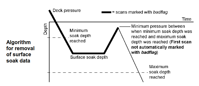
It is possible - and occasionally necessary - to modify any of the parameters involved in the SBE processing operations, or the combinations of operations themselves. This document doesn’t contain information about the details of the SBE processing (look for them in the Seasoft V2 Data Processing Software Manual), but one common modification is changing the surface soak depth parameters in the Loop Edit processing step. These parameters are used to identify and remove the part of the profile where the CTD is “soaked” at an initial depth, typically 20-50 m, before the profile begins. (Soaking is done to activate the conductivity pump -the CTD is subsequently brought up to right below the surface and then the actual downcast profile begins).

The SurfaceSoakDepthMin/Min parameters in LoopEdit.psa specify a pressure range within which the CTD is stopped to soak before being brough up again. Problems typically occur if the CTD was soaked at a depth outside this range. You may see this as messy data (especially conductivity/salinity) in the upper tens of meters as the profile includes parts of the cast where the conductivity pump was not turned on.

The solution to this is typically to:

Identify the actual soak depth (how deep did the CTD go before being pulled up to the surface to start the cast).

Modify the SurfaceSoakDepthMax and SurfaceSoakDepthMin parameters in LoopEdit.psa.

You can do this in a text editor, or in the SBE software - see page 103 of the SBE Processing Software Manual.

Note that there is also a parameter just called SurfaceSoakDepth - this doesn’t seem to actually do anything.

Rerun the SBE processing, producing updated .cnvs.

For example, if your LoopEdit.psa specified SurfaceSoakDepthMax=15 and SurfaceSoakDepthMax=25, but the CTD for some reason was soaked at 30 m, you will very likely see junk in the top of your profile. You should make sense that the SurfaceSoakDepthMax parameter is greater than 30 (something like 35 might be good), e.g.:

<SurfaceSoakDepthMin value="15.000000" />

<SurfaceSoakDepthMax value=" ~~25.000000~~ 35.000000" />

9. Setup your python environment and fire up JupyterLab

We now need to install the Python packages necessary to run the post-processing. This includes JupyterLab (a web-based interactive development environment for notebooks, code, and data) and NPI’s Python libraries kval (Python tools for processing and analysis of ocean data), and naust (NPI-specific tools and templates).

The easiest way to do this is to install a pre-made conda environment where everything has been set up for you. To do this, run this in your a conda-enabled terminal like Miniforge (from the root directory of your repository - where you should have a file ctd_env.yaml):

conda env create -f ctd_env.yaml

This installs a Python environment ctd_env with compatible versions of kval, naust, jupyter, and other required libraries.

To work within this environment, activate it in your conda terminal:

conda activate ctd_env

.. and while we’re at it: register the kernel in Jupyter (never mind what this means for now; also not strictly necessary) by pasting the following into your terminal

python -m ipykernel install --user --name ctd_env --display-name "CTD conda environment"

You can now start up JupyterLab and begin working with notebooks:

First, activate the conda environment (or another environment with all requirements installed): conda activate ctd_env
Navigate to your root project folder, and start Jupyter Lab: jupyter lab
This should open a window in your browser. You can now browse in the folder structure using the left side menu, open existing notebooks or files, or create new ones.
When running a notebook, you can specify which Python kernel to use. For CTD processing, you should select the CTD environment we created earlier (or another environment with all the requirements installed):
- Click Kernel -> Change kernel.. in the top menu.
- Choose CTD conda environment (this option should be available if you registered the kernel - enabled JupyterLab to see your conda environment - in #9)

10. Perform salinity QC

If salinity samples were collected during your cruise, laboratory salinity values should be compared with CTD-derived salinity values (from .btl files produced in Step #8). Salinity from water samples first have to be measured using a salinometer (see this).

If you have all the necessary inputs, you should be able to do this by opening JupyterLab (see #9) and running a few lines in code/salt_qc/Salinity QC.ipynb
More detailed instructions here: QC of CTD salinity data

11. Calibrate oxygen/Chl-A/etc

To obtain high-quality CTD data on Chlorophyll-A, oxygen and other parameters, the CTD-derived values typically need to be calibrated against in-situ samples that have been processed in the lab (filtering and chl-a measurements, winkler titrations).

Typically, this amonts to something like a linear fit based of laboratory values against CTD measurements at bottle closure (.btl files). There are no detailed instructions for how to do this here.

The outcome of such a laboratory calibration is typically:

A mapping used to convert uncalibrated CTD values to calibrated values (e.g. \(x_2 = Ax_1 + b\)).
- Will be applied to the data.
A description of how the calibration was done.
- Will be applied to the dataset metadata.

In some cases, an additional correction is applied to compensate for non-photochemic quenching using transmissometer attenuation data (see Thomalla et al. 2017). In this case, you will have to format the metadata accordingly.

12. Inspect the data

Use JupyterLab to run the notebook code/ctd/1. Inspect CTD.ipynb.

Note: Make sure to run with an appropriate kernel. If you installed the conda environment ctd_env.yaml and registered the kernel in Step 2:
- Ckick Kernel -> Change kernel.. in the top menu.
- Choose CTD conda environment

Running this notebook doesn not modify anything, but should make sure data can be loaded and give you a good overview of what’s in the data.

In this notebook, we:

Try loading the data from .cnvs to an xarray dataset.
Plot a quick map of the CTD stations as a sanity check.
Produce dynamic contour plots of the CTD profile data - useful for getting the feel of what we are measuring.
Inspect individual profiles (you should visually inspect all profiles you intend to publish at least once!).
Plot variables agains each other (plot in “phase space”) - e.g. T-S diagrams - to dig a bit deeper into anything you find suspicious.
Compare dual sensors (e.g. dual conductivity sensors) to identify issues or offsets between the two.

For anything not covered by the statndard kval functions, you may want to create your own plots. Look up basic python/matplotlib syntax - it’s not too hard even if you’re not familiar.

It is good to make some notes in the notebook (at the bottom of the notebook for example), summarizing your impression and noting down any specific problems. This will be useful in the rest of the process.

13. Edit the data

Run the notebook code/ctd/2. Edit CTD.ipynb. In this step, we load the data from .cnv files to an xarray Dataset, perform some operations, and save to a temporary NetCDF file.

In this notebook:

Load the data from .cnvs to an xarray dataset.
Apply any corrections, e.g.:
- Inspect disctribution of values and apply thresholds for valid data if necessary
- Apply fixed offsets if that has been deemed necessary besed on other analysis
- Apply (linear) chlorophyll calibration based on comparison between fluorometer and in-situ values.
Edit outliers
- This is typically necessary at least for salinity, where we usually have some spikes due to particles in the conductivity cell.
- The hand_remove_points() function helps you edit out these points by hand.
Save to a temporary NetCDF which we will load in the final post-processing step.

You may want to also execute any other code used to modify data in this notebook (we will deal with metadata in the next one).

14. Finalize the file and metadata

Run the notebook code/ctd/3. Finalize CTD.ipynb. In this step, we load the NetCDF file produced in the previous step, and make changes to the file structure and metadata until we are happy with it and everything is compliant with CF/ADCC conventions.

In this notebook:

Load the data from .nc produced in step 12.
Remove any variables we don’t want to include in the final dataset.
Import metadata attributes from metadata/CTD_global_metadata.yaml and metadata/CTD_variable_metadata.yaml (see Step 6).
Automatically add some metadata based on the data (geospatial and temporal ranges, standard attributes, keywords etc).
Add a date_created attributebased on today’s date.
Convert all 64-bit floats and ints to 32-bit - recommended for robustness across syetems.
Convert any NaNs to numerical fillvalues (default -9999) - recommended for robustness across syetems and to minimize ambiguity.
Run some checks:
- Run the IOOS CF-convention checker
- Run a custom, complementary checker in kval
  - Covers some common issues not covered by the IOOS checker
- Note: These checkers are very useful, but they don’t catch everything. You should also be checking carefully yourself!
Produce a final, well-formatted NetCDF file.
- In principle, this shoudl now be publication-ready, in practice you may want to return to update tweak things, e.g. after reaching out to coauthors or double checking.
Optionally also export a .yaml file mirroring the contents of the NetCDF, and a .mat file if you have collaborators that prefer that.
- What you shoudl publish is the .nc file.

In practice, you will probably want to work iteratively here. Make some changes, encounter something weird further down, go back and modify something, run a checker, modify somethign else flagged by the checker, etc.. When you pass the checkers without any major issues and you have looked thorugh the data and metadata yourself, you probably have a really well-formatted NetCDF.

At this stage, you may want to share your NetCDF, and the associated .yaml file, with collaborators to make sure everyone involved is happy with the file and metadata. You can always come back to this notebook and make changes.

14. Upload your files to data.npolar.no

Go to your data.npolar.no dataset landing page -> Edit -> Files. Here, you may Add individual files or Add directory to add an entire folder (useful for raw data).

Good to upload both the netCDF file produced in step 13 and a folder containing the source SBE files (e.g.: source/raw for .hex, .xmlcon and source/human_readable/ for .cnv, .btl).
Optional: also include the notebook/script to reproduce the processing

Note you can delete uploaded files and make other changes until the dataset is published. When the dataset is public, you can not remove or modify the uploaded files (however, you can upload newer files, e.g. _v2.nc).

15. Look over the dataset page

Are the correct files uploaded?
Is the landing page information and metadata information (time span, geographic area, dataset description, keywords, authors..) correct?
Are things set up such that you can easily upload a newer version if the data if you need to later?
Are the correct links (to cruise reports, projects etc) in place?

16. Make the dataset public

When you are happy with the data and metadata, and have double checked everything:

Go to your data.npolar.no dataset landing page
Click Publish, and Ok to confirm.
- This will
  - Activate the dataset DOI
  - Make the dataset publicly visible (no login required).
  - Lock attached files in place (they can no longer be removed).

Hooray!

Nice

17 (for KPH): Communicate files to IMR

IMR will integrate processed KPH CTD data into Copernicus, data repositories used for generating ocean climatologies, etc. Notify them about the finalized dataset. (Contact Helge Sagen).

18. Clean-up

When you are done, you should:

Clean up the Gitlab repo (especially: undate README.md).
- Your goal shoudl be to help someone else (or yourself in the future) understand what goes on in the repository.
Delete the ctd_env conda environment:

conda env remove -n ctd_env
- Not necessary, but good practice. Also prevents any confusion next time you want to install this environment from ctd_env.yaml (which may be updated later).
If anything in the process, scripts, or instructions felt confusing or clunky, just send a quick message to Øyvind. Feedback is super helpful and will help make this process easier next time someone does it.
Pat yourself on the back, and notify collaborators or any other interested parties that the dataset is publicly available.