QC of CTD salinity data#
Related:
Inputs#
To perform the salinity QC, you need three main inputs:
.btlfiles from the CTDContain salinity measured by the SBE CTD unit at bottle closure.
Produced from raw data (
.hex,.xmlcon,.bl) as part of the standard processing in SBE Data Processing (which also generates.cnvfiles).Values in the
Stationfields (entered by the CTD operator during CTD mesurements) should be compatible withSTATIONvalues in the water sample log. In some cases it may be necessary to edit theStationfield in the.btlfiles.
File with salinometer readings
Contains the final values from salinometer measurements.
Final lab salinity is typically the median of 3–5 readings, corrected with an offset based on calibration against standard water of known salinity.
Usually handwritten during lab measurements and later digitized into an Excel sheet.
Log sheet template for handwritten values:
logsheet_salinometer.pdfExcel template for digitization:
salinometer_readings_template.xlsx
See Salinometer guidelines for details on laboratory measurements.
Log sheet for CTD water samples
Links bottle sample numbers (identifying each salinity bottle / each lab salinometer value) to corresponding CTD station and Niskin bottle numbers.
Two formats are in use at NPI:
Fram Strait-style log sheet:
CTD_sample_log_FS_style.xlsxrows = Niskin number / columns = CTD station
Troll Transect-style log sheet:
CTD_sample_log_TT_style.xlsxrows = water samples
Both formats work and can be parsed using
naust.salts.
General steps#
Combine readings and CTD sample log
Match each lab salinity reading to a CTD station and Niskin number using the salinity sample number as a common reference.Combine with CTD salinity from
.btlfiles
Use station and Niskin number to pair lab salinity with CTD salinities measured at bottle closure.Compute differences between CTD and lab salinity
Calculate differences between lab and CTD salinity for each sample (separately for primary and secondary sensors,PSAL1,PSAL2if available).Analyse the differences
Create histograms of salinity differences, scatter plots comparing lab and CTD salinity, etc.
Exclude samples from the upper water column where strong gradients dominate.
The depth limit is somewhat subjective and depends on the cruise and regional stratification.
Common minimum pressures: 250, 500, or 700 dbar.
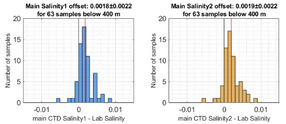
Example plots of distribution of lab-CTD differences for primary and secondary salinity (a case where the QC test passes):
Conclude
In general, the mean or median CTD–lab difference should not exceed 0.003 PSU.
If within this bound, the “quality test” is usually considered passed.
Always check the data carefully—averages can mask important patterns.
Additional checks:
Spread of distribution:
A narrow distribution centered near 0 ± 0.003 PSU is expected.
Outliers dominating the mean but not the mode may still give confidence in CTD salinity.
A wide spread, even if the mean looks good, reduces confidence.
Time evolution of offsets:
Watch for progressive sensor drift during the cruise (e.g., due to biofouling, freezing, or mechanical issues).
For CTDs with duplicate sensors, compare the CTD–lab salinity differences of
PSAL1andPSAL2.This can guide which variable to use in scientific analysis and published datasets.
If we consider the QC test as “passed”#
We can trust the CTD values and can proceed to use the salinity values in the
.cnvfiles as a starting point for post-processing and data publising/scientific use.It should be indicated in documentation and metadata that the salinity data have been quality controlled against laboratory saliity measurements.
I may also be useful to give more details, e.g.:
Include diagnosis plots in processing reports, etc.
Indicate the spread of the observed differences (SD, e.g.) as it can give an indicatin of the data precision.
Note that additional post-processing (outlier editing, etc) still needs to be applied before the data are ready for scientific use!
If we consider the QC test as “failed”#
Before concluding and/or taking action, it is good to double check the results.
E.g. manually confirm that we are comparing the right values for a few samples.
If differences are systematic, you may be able to correct for them by applying a “calibration correction” to the data.
Preferably, corrections should be applied to conductivity (salinity can then be recalculated from C/T/P).
Corrections to conductivity should generally be applied as a scaling factor, not an offset.
You may also want to check that CTD sensors have been recently calibrated - and consider having a new calibration performed after the cruise.
If CTD salinities calculated using new calibration coefficients perform better, you may want to use these coefficients to prduce the scientific data.
If the results are conclusively bad, you may be dealing with a bad sensor, and it may simply not be possible to use the data.
Helper scripts in naust (Python)#
The procedure above is completely generic, and you may code this up however you want. For those interested, a helper Python module has been created in the naust library (salts.py).
Contains functions to parse, combine, and analyse datasets with a few lines of code.
Should work with standardized input formats.
If you diverge significantly from the templates above, you are likely to encounter problems.
Minimal example:
from naust import salts

# Locate input files
salinometer_sheet = 'salinometer_readings_my_cruise.xlsx' # Parsen salinometer readings
ctd_log_sheet = 'CTD_sample_log__my_cruise.xlsx' # Should tackle both TT and FS formats
btl_dir ='btl/' # Directory containing .btl files

# Combine all three inputs into one single structure and compute salinity differences
ds_sal = salts.build_salts_qc_dataset(ctd_log_sheet, salinometer_sheet, btl_dir)

# Some standard analysis plots
salts.plot_by_sample(ds_sal)
salts.plot_salinity_diff_histogram(ds_sal_qc, psal_var='PSAL2', min_pres=200)
salts.plot_scatter(ds_sal_qc, psal_var='PSAL1', min_pres=500);